Predicting coordinates
After creating the GeoClassiffr that predicts the country in which an image was taken, I wanted to make a model a bit more interesting, by training it to predict the coordinates where an image was taken. This turned out to be quite a bit tougher, but after much tinkering I am quite happy with the model, especially since I believe performance can improve further by scaling up the training data and the number of model parameters
You can find the model code, training code, and dataset creation code all on my Github.
Dataset
The model was trained on a custom-made dataset containing ~300,000
unique, high-quality Google Maps images and their associated coordinates. This data was gathered using a
script that automatically plays GeoGuessr rounds, takes a screenshot and extracts the
associated coordinates. I did this process for various maps, so the overall distribution is a mix of
official country/world maps, as well as user-generated maps of more unique or underrepresented locations,
for example.
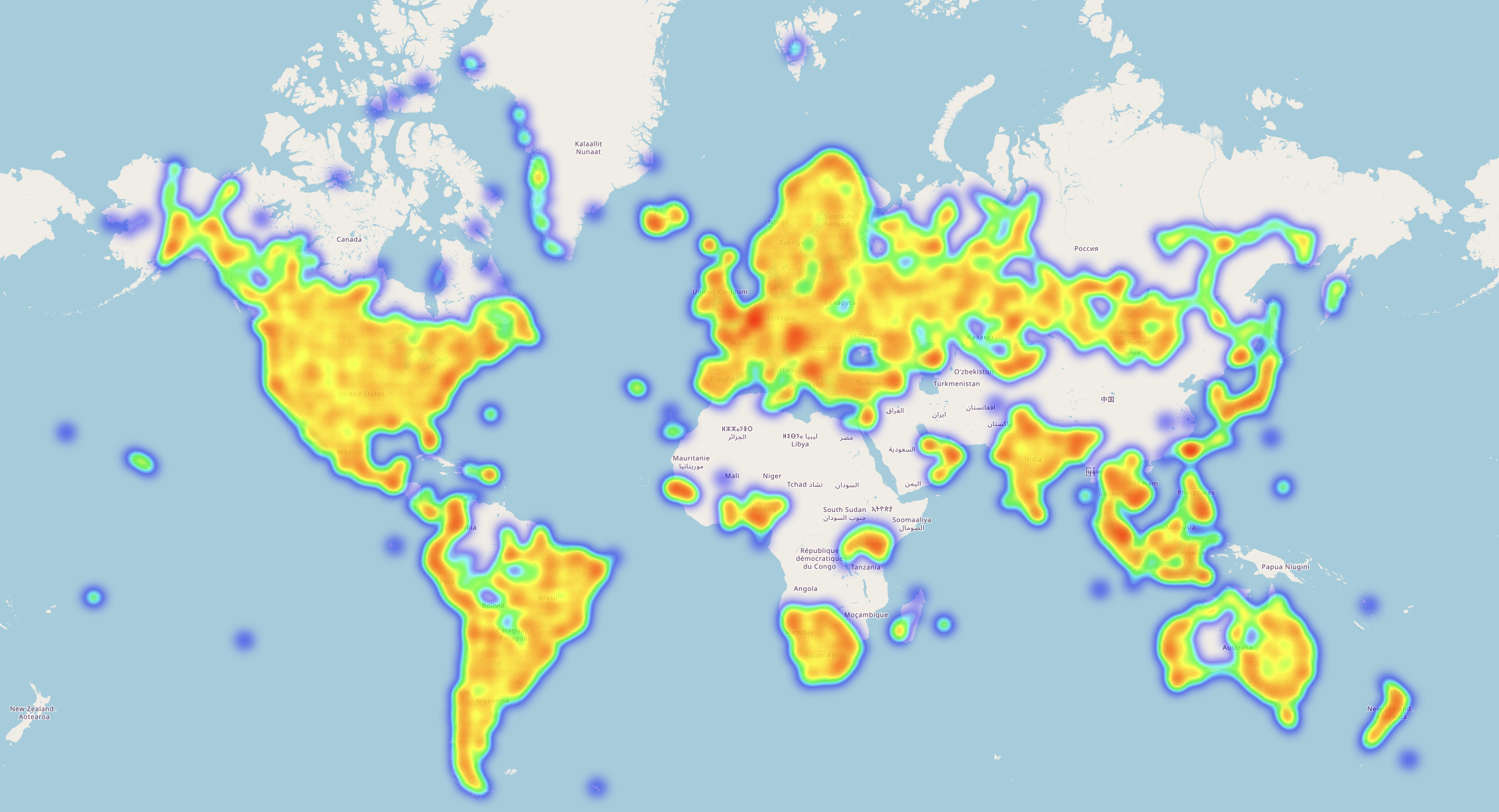
As can be seen in Figure 1, most of the world is included. Notable exceptions are Africa, much of the
Middle East, China and parts of Northern Canada.
See Table 1 for an overview of the distribution of train set locations. The test and validation sets have
an identical distribution (within 0.1%).
Notably, the USA is quite over-represented, accounting for roughly 13% of all images.
Continents
| Continent | Count | Percentage |
|---|---|---|
| Europe | 73,125 | 32.09% |
| Asia | 50,838 | 22.31% |
| North America | 47,510 | 20.85% |
| South America | 29,566 | 12.98% |
| Africa | 17,146 | 7.53% |
| Oceania | 9,652 | 4.24% |
| Antarctica | 15 | 0.01% |
Top 10 Countries
| Country | Count | Percentage |
|---|---|---|
| United States of America | 29,395 | 12.9% |
| Brazil | 8,981 | 3.94% |
| Russia | 8,923 | 3.92% |
| Canada | 8,108 | 3.56% |
| Australia | 6,784 | 2.98% |
| Mexico | 6,350 | 2.79% |
| Indonesia | 6,007 | 2.64% |
| France | 5,967 | 2.62% |
| Argentina | 5,553 | 2.44% |
| Japan | 5,528 | 2.43% |
Model architecture and training
I used a DINOv3 backbone MoE architecture, with each head regressing spatial locations directly onto a 3D unit sphere rather than predicting raw latitude and longitude. Direct regression of latitude and longitude introduces boundary discontinuities at the ±180° meridian and numerical instability near the poles, which led to training plateauing prematurely. To eliminate these edge effects, the network maps ground-truth coordinates (ϕ,λ) to a 3D Cartesian unit vector (x,y,z)=(cosϕcosλ,cosϕsinλ,sinϕ).
To handle the visual diversity across different continents and biomes, the model uses a Mixture of Experts architecture. The learned gating mechanism routes the representations of each input image to the top-k specialized expert networks. The final coordinate prediction is then a sparsely weighted combination of the selected experts' outputs.
To actively guide this routing and encourage expert specialization, the architecture incorporates an auxiliary classification task based on S2 geometry. S2 cells hierarchically partition the Earth's surface into discrete geographic regions. By requiring the network to simultaneously predict the discrete S2 cell corresponding to the location, the model receives a strong, coarse-grained geographic signal. This auxiliary task acts as a structural hint for the MoE gating mechanism—driving it to cluster geographically and visually related images together, allowing the individual experts to specialize in specific regional domains while the direct 3D regression fine-tunes the exact local placement.
The model was trained using a weighted sum of the Mean Squared Error loss between the predicted and target 3D unit vectors, an S2 cross-entropy loss and a load balancing loss. Because the Euclidean distance between two unit vectors is monotonically related to their great-circle distance, optimizing MSE in 3D space effectively minimizes spatial chord distance on the surface of the Earth without coordinate singularities.
Because I had limited compute available, I ran a hyper-parameter sweep on the vit-s+16 backbone. Once I found optimal parameters, I trained a vit-b16 backbone model, as well as a vit-l16 backbone model. I only trained for 16 epochs, meaning the models had not converged yet (again due to limited compute). Still, the results are not bad, meaning they will only get better with more data and compute.
Model analysis
All in all, all three models performed better than I would have initially expected. Table 2 displays the medium-sized model's distance and GeoGuessr score on the test set. The GeoGuessr score is based on the distance, with the same multiplier used in the 'world' maps. As can be seen from the Table, the model excelled at guessing Europe and North America. This is no surprise, given a large part of the dataset covered these two continents, due to the fact that the majority of Google StreetView coverage is in these places. Africa, remarkably, has the largest spread between good and bad guesses. While average distance is definitely not among the best, the 20th percentile distance is the best out of all continents, and the 80th percentile is among the worst. This is most likely explained by the sparse coverage of StreetView in Africa. Because there are not many places in Africa that are possible, whenever the model guesses Africa, it is likely to be fairly close to the true place. Despite this fact, much of Africa can be quite ambiguous, with common clues such as red sand soil and jungle-like foliage also being common in places like Brazil/ Australia or South America/ Southeast Asia, respectively.
Results by Continent
| Continent | Samples | Dist Avg (km) | Dist p20 (km) | Dist p50 (km) | Dist p80 (km) | Score Avg | Score p20 | Score p50 | Score p80 |
|---|---|---|---|---|---|---|---|---|---|
| Africa | 2033 | 1490.8 | 191.5 | 435.7 | 1765.0 | 3372 | 2069 | 4021 | 4543 |
| Asia | 5772 | 1337.2 | 262.3 | 577.1 | 1315.4 | 3396 | 2590 | 3747 | 4385 |
| Europe | 8475 | 711.0 | 225.1 | 445.1 | 841.3 | 3773 | 3283 | 4002 | 4468 |
| North America | 5946 | 1168.5 | 246.3 | 499.7 | 1135.6 | 3492 | 2834 | 3895 | 4421 |
| Ocean/Unknown | 1643 | 1995.9 | 294.0 | 704.5 | 2058.0 | 3043 | 1787 | 3515 | 4316 |
| Oceania | 1116 | 2179.9 | 265.6 | 599.7 | 1779.6 | 3178 | 2054 | 3705 | 4378 |
| South America | 3498 | 1635.2 | 275.9 | 640.7 | 1583.6 | 3223 | 2265 | 3630 | 4356 |
| Overall | 28483 | 1234.2 | 242.7 | 512.6 | 1197.4 | 3476 | 2748 | 3870 | 4429 |
MoE analysis
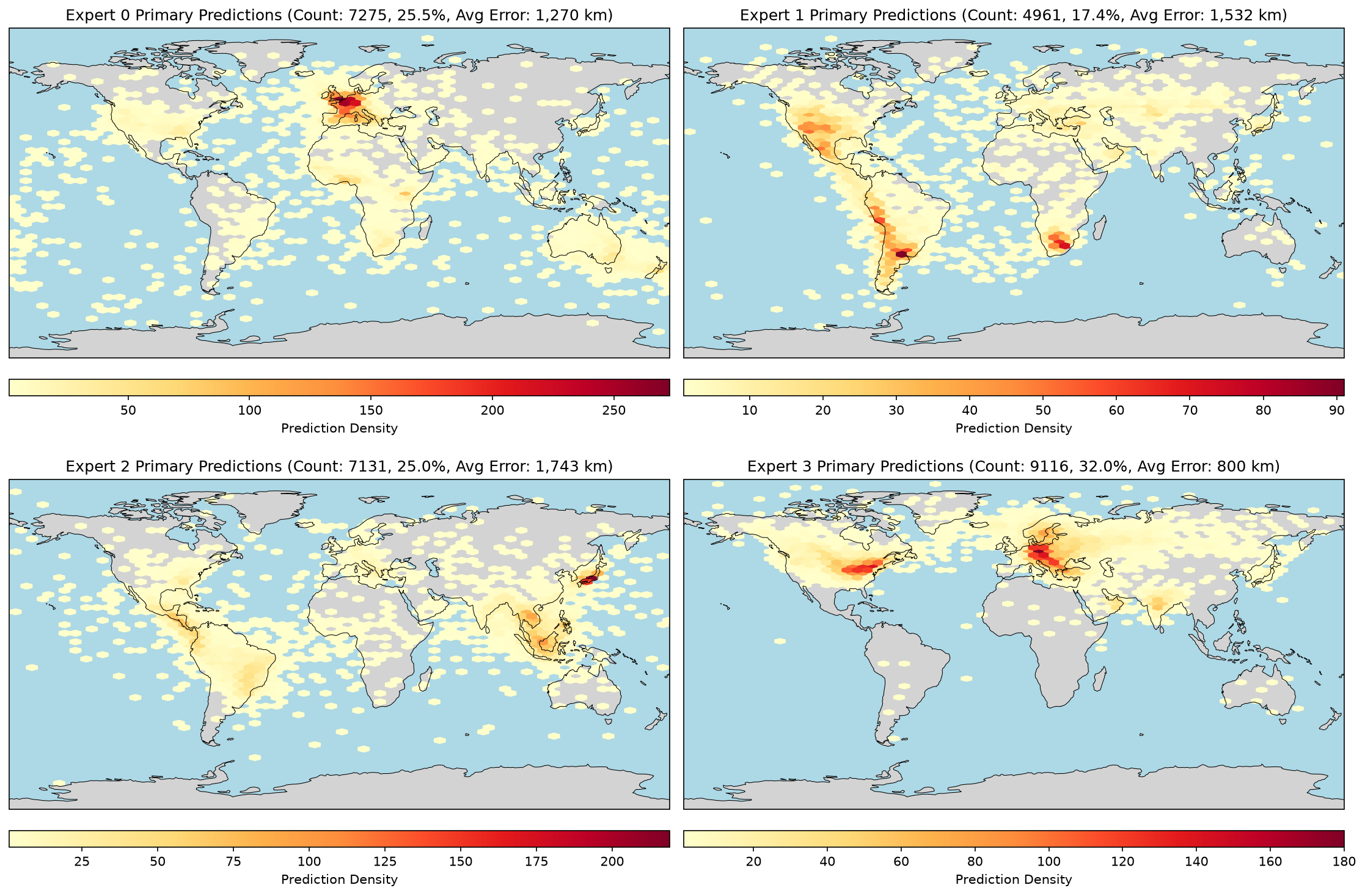
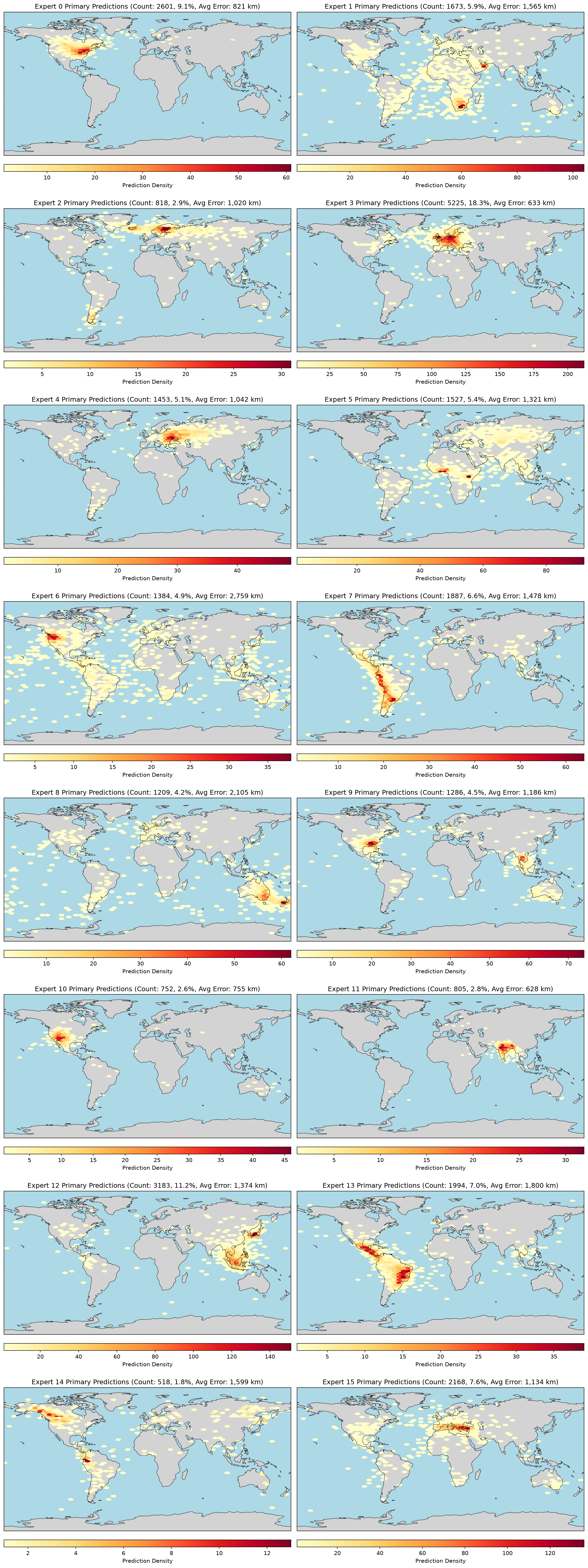
Figure 2 below displays a heatmap of the locations each expert has guessed on the test set. Indeed, the different experts are each responsible for their own geographic area. Figure 2 displays the heatmaps for the vit-b16 backbone model with 8 experts. See the appendix for the heatmaps plots of the model trained with 4 and 16 experts.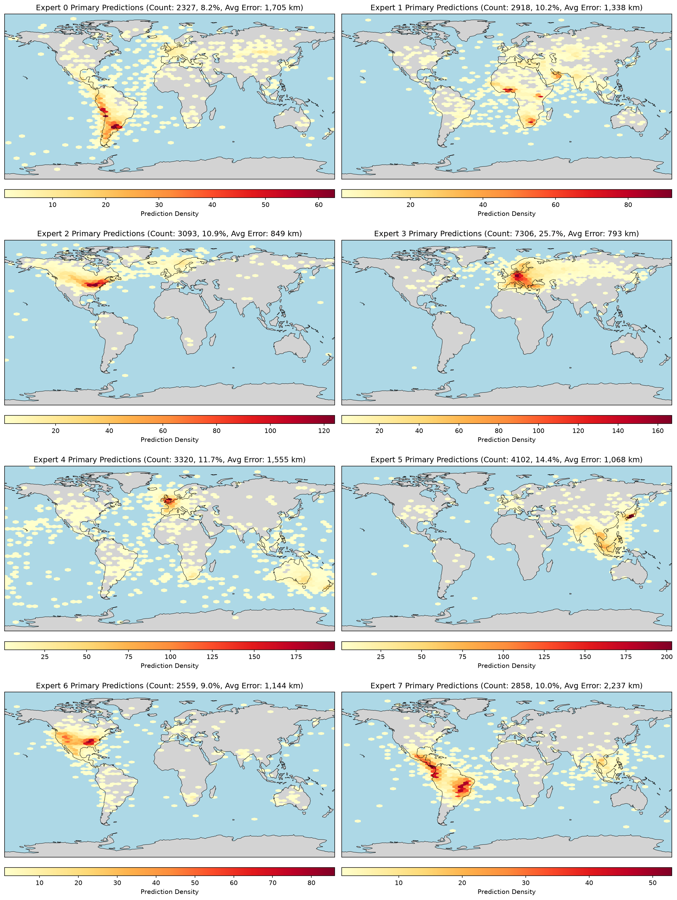
Common mistakes
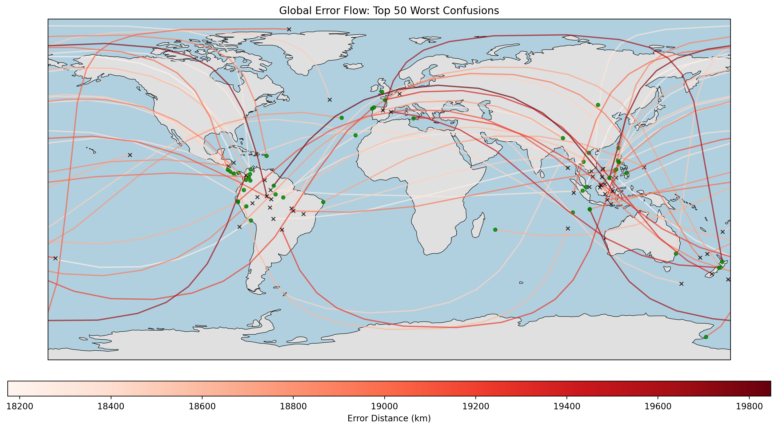
Figure 3 shows the 50 worst mistakes made by the vit-b16 backbone model with 8 experts. As we can see, most of these locations' true or predicted coordinates are in Southeast Asia and South America, primarily in the forested areas of the two. We can indeed see, in Figure 2 expert 7, that these locations are both in that expert's prediction domain. Perhaps increasing the number of experts reduces the probability of these mistakes, as the probability of an expert being overextended would be lower.
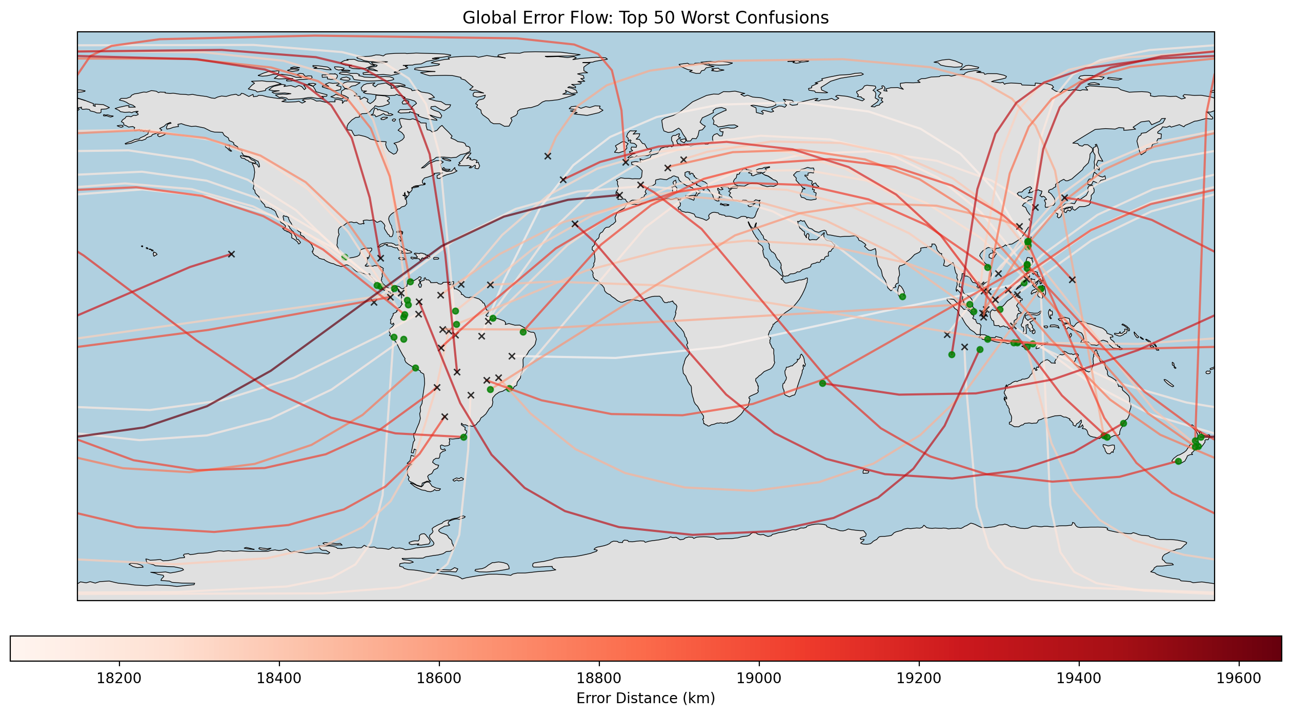
When we make the same plot for the same model, but with 16 experts, we see that this is not the case. In fact, the model makes almost the exact same mistakes, indicating that indeed, these locations are simply too difficult for the model to predict accurately.
Below are some images from the test set, along with their predicted and true coordinates. In Figure 5, the model predicted the correct jungle and mountain range, being accurate within 120km and 170km, respectively. The exact coordinates in these situations are quite ambiguous, as a jungle or mountain range inherently looks visually uniform, and stretches for hundreds of kilometers.
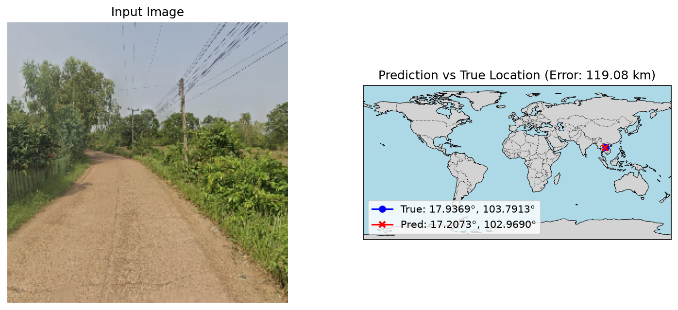
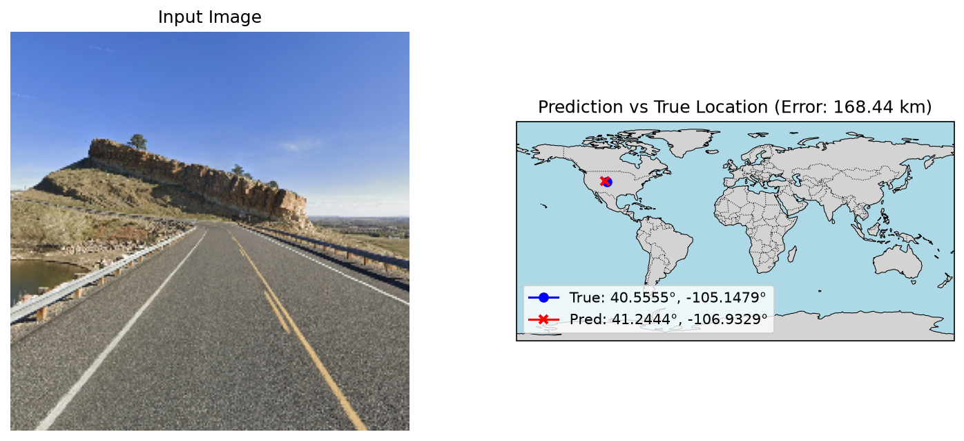
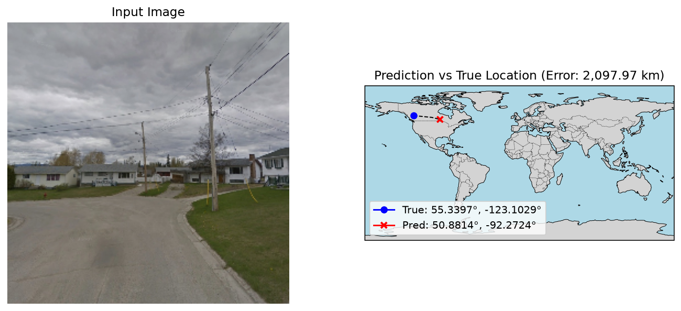
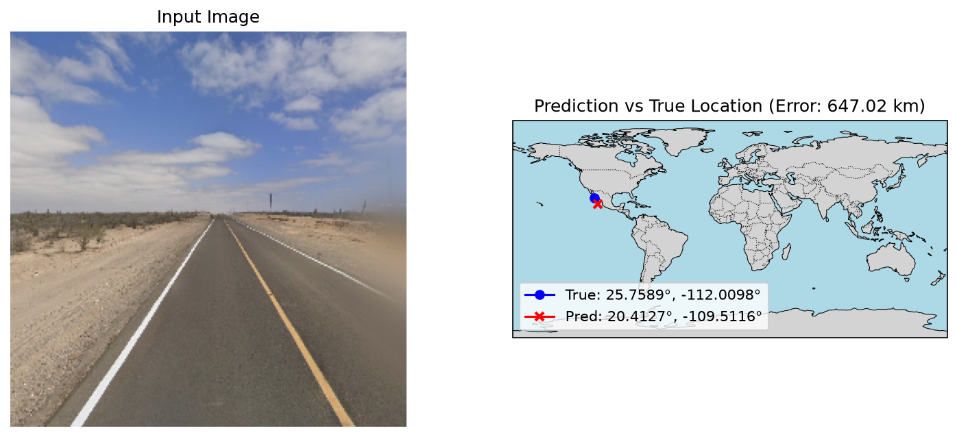
Figure 6 shows some worse predictions, though the mistakes are explainable and not too 'stupid'. The top
image is simply a less-wealthy, rural, Canadian suburb. This image could realistically be taken in most
parts of Canada, with nothing in the image that gives away the fact that it should be in British Columbia
specifically.
The same is true for the bottom image. It is not too difficult to deduce that it was taken in Baja
California, Mexico. The specific location in Baja California however is less obvious, and
unfortunately it is a large place.
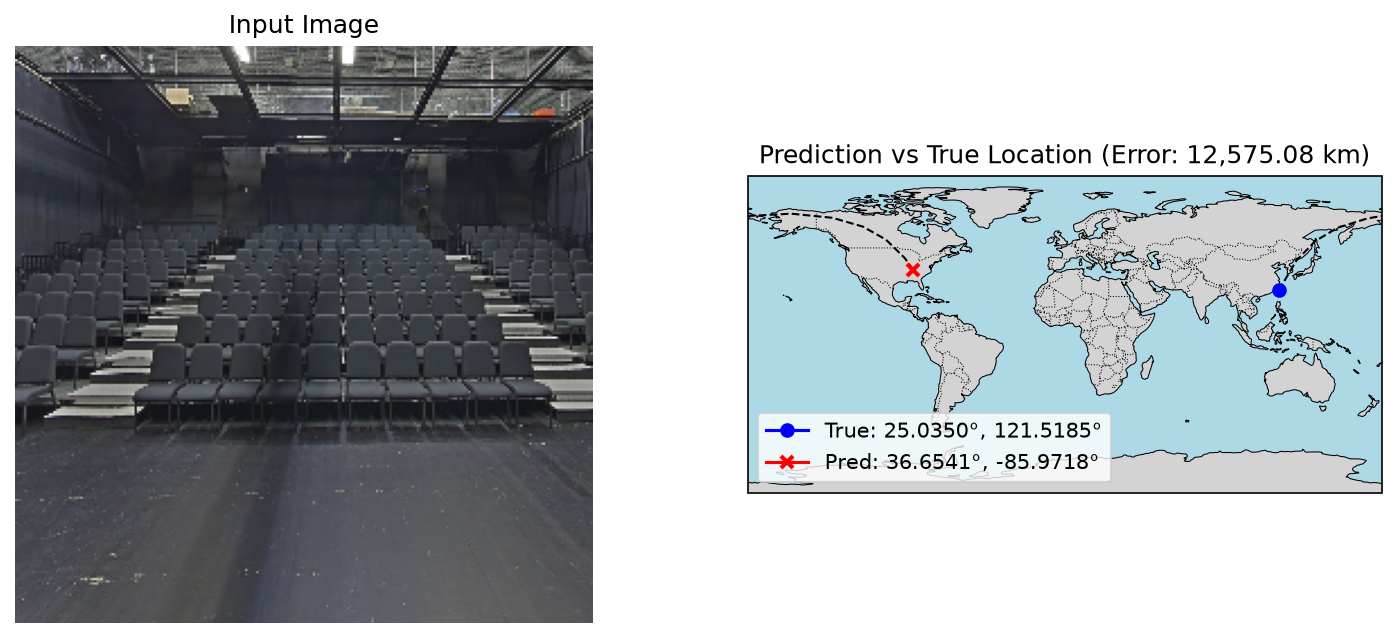
Lastly, Figure 7 shows an example of why the average is a bit skewed. Sometimes in GeoGuessr, you get indoor locations. For humans, such locations are quite easy, as there is often some language or people visible that help you deduce the location. For our model, however, such situations could be anywhere, so the prediction is more like a random guess.
Attention analysis
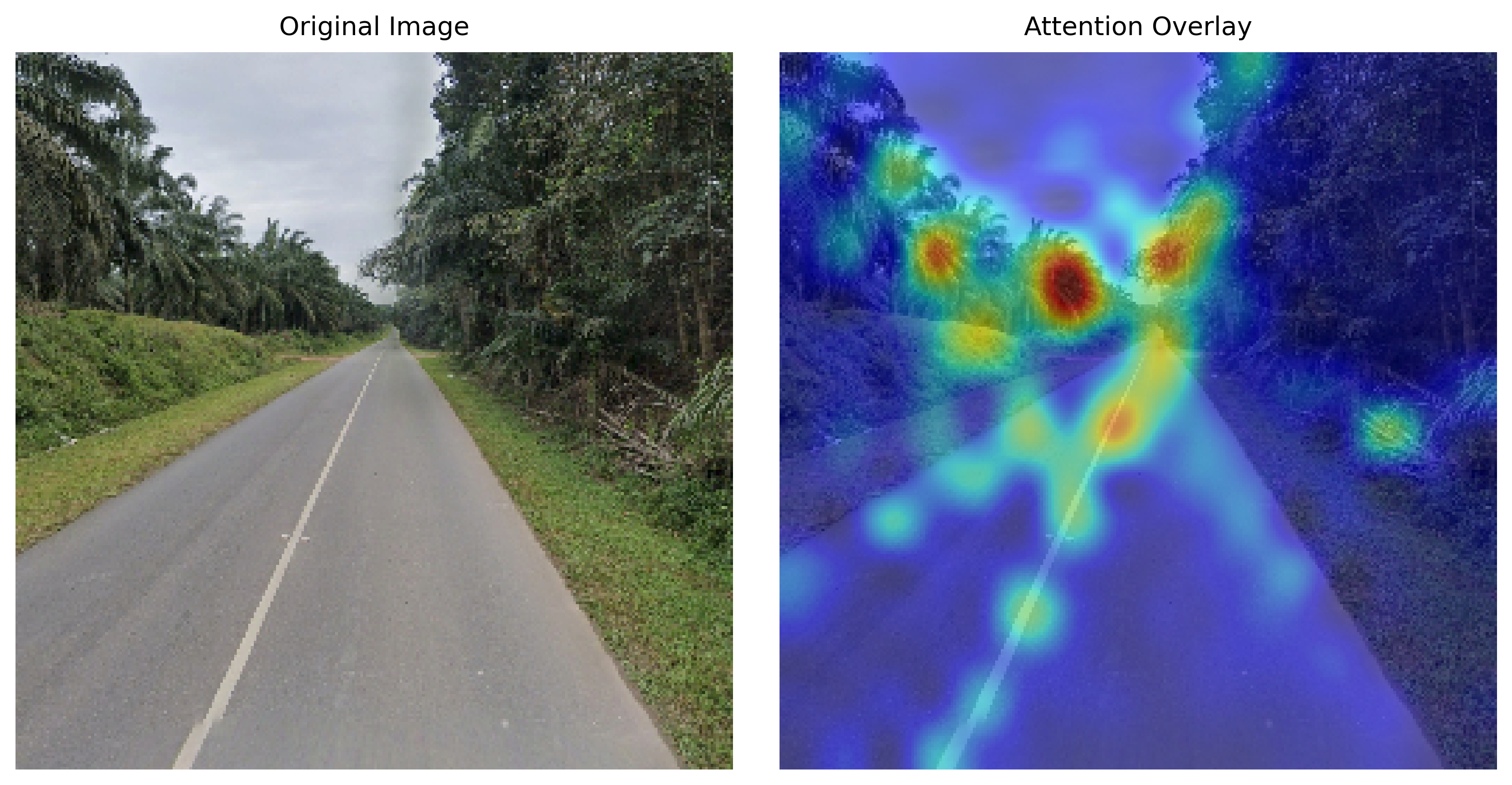
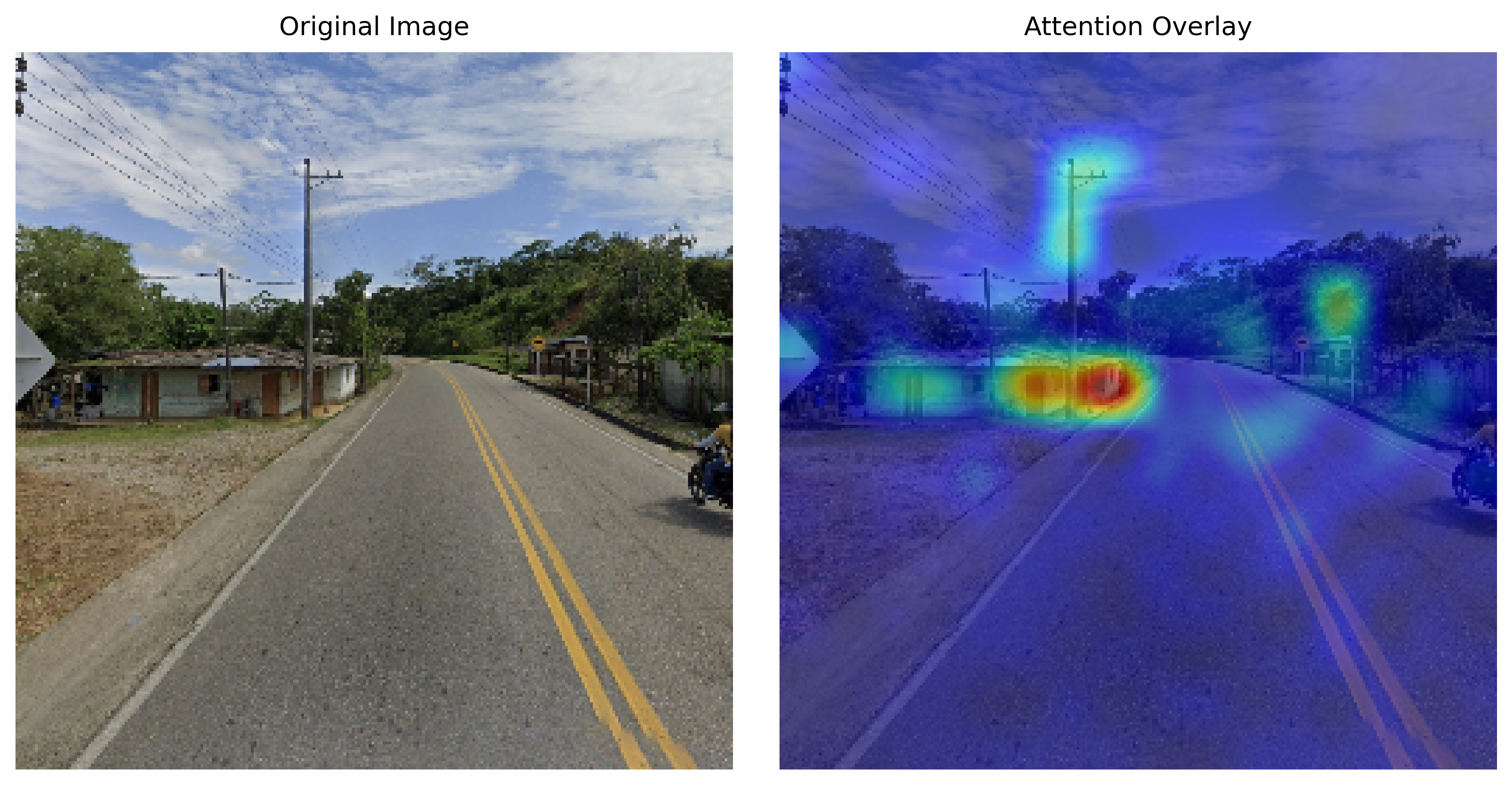
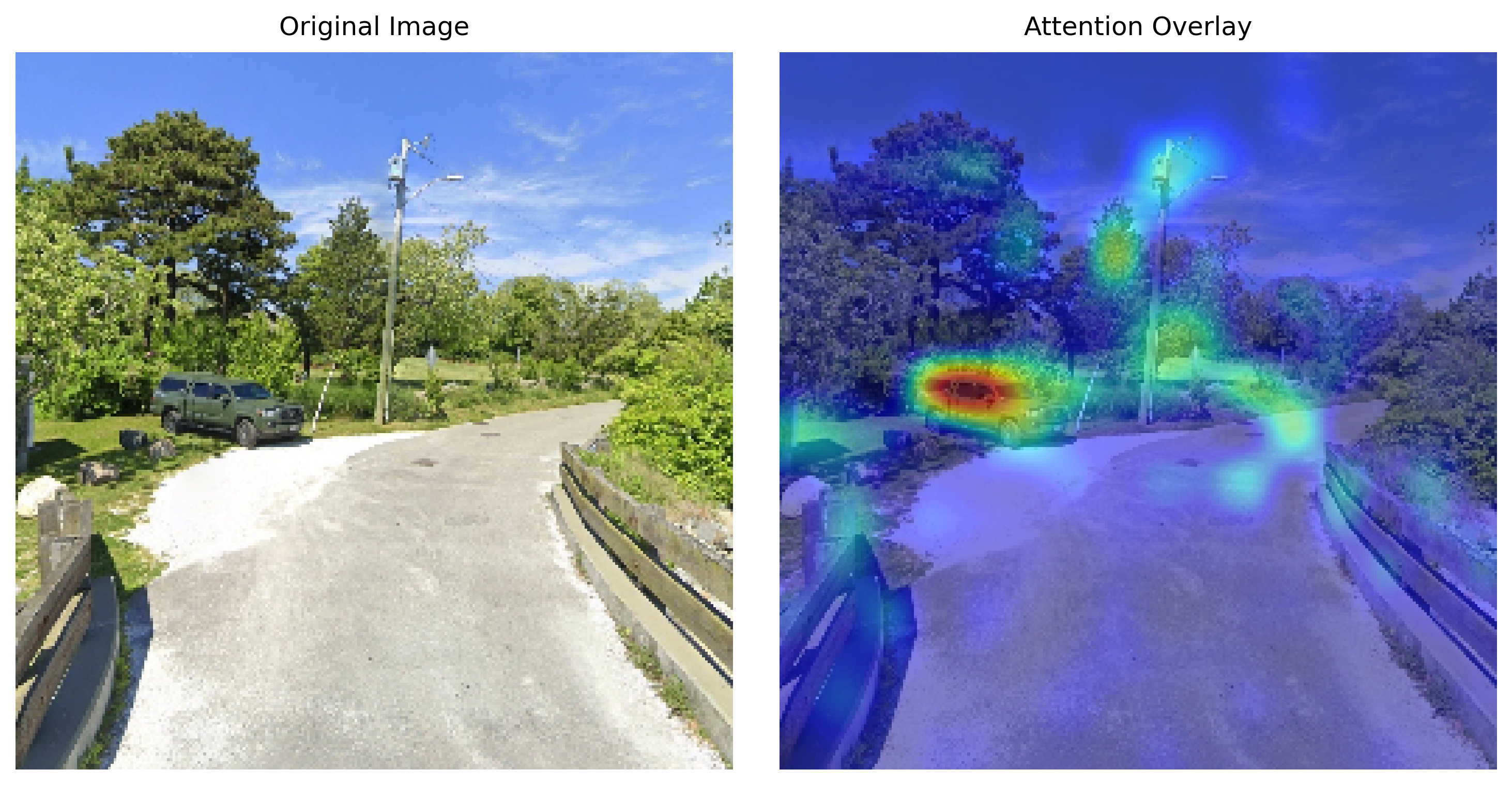
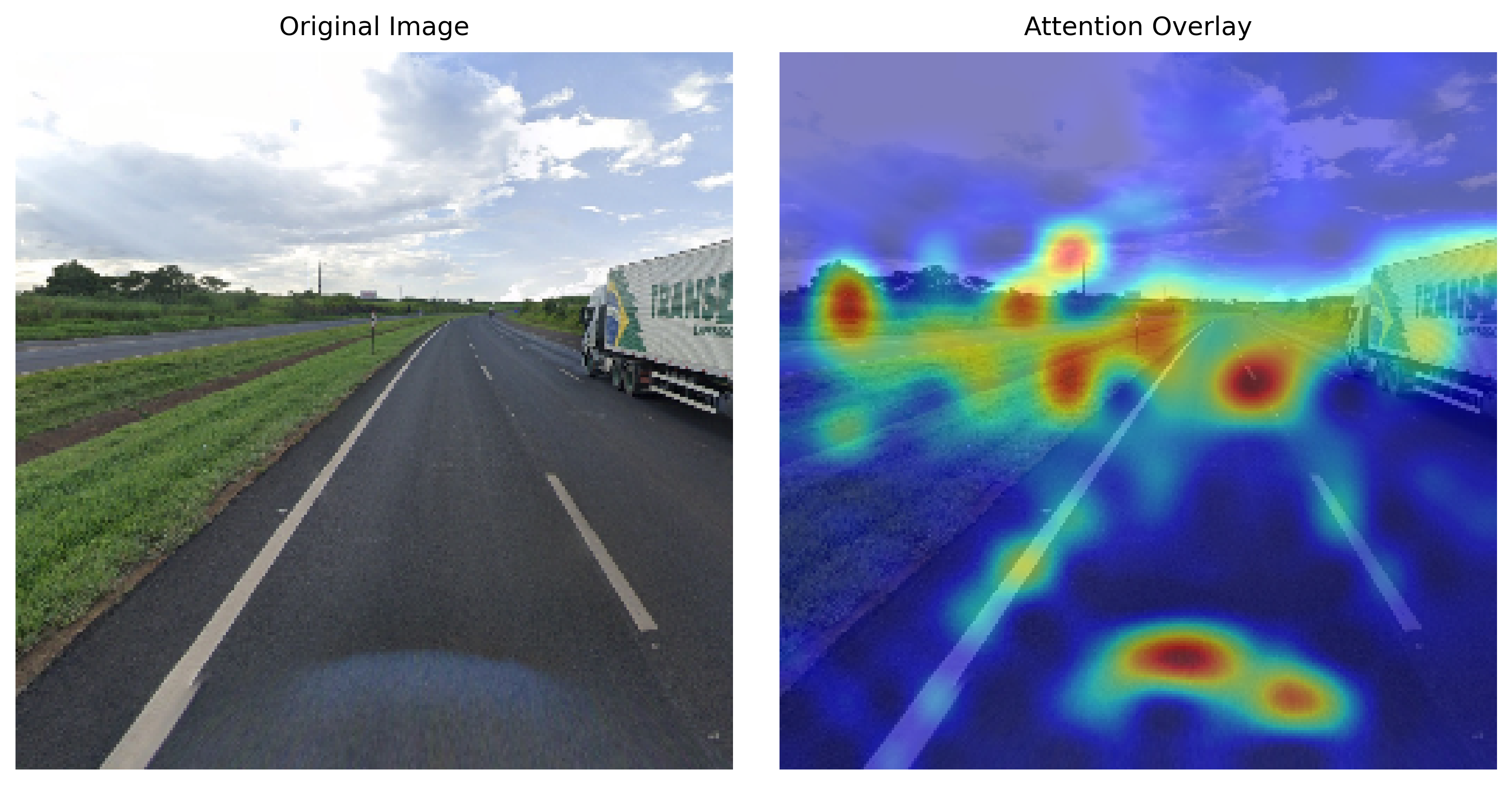
Figure 8 displays the self-attention of the trained model. As we can see, the model learns to focus on roughly the same clues a human would focus on when playing GeoGuessr: road lines, road signs, (utility) poles, cars, houses/architecture, foliage and trees.
Future work
As we concluded from Figure 3 and 4, certain areas are clear weak points for the models, leading to an obvious solution of gathering more datapoints for such geographical areas. This is quite low-effort as the dataset generation script is already there. I currently do not have the time however (and my GeoGuessr subscription has expired).
To gather more train data, I think finetuning a GAT model specifically for underrepresented countries would lead to the model being better at distinguishing such countries. Unfortunately, I did not have the computational resources to test this hypothesis, but perhaps in the future I will try.
Appendix
MoE analysis